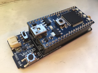
Instructions and troubleshooting for the VertigoIMU inertial datalogger.
Born
to Engineer films from the ERAF
Lessons Available
Physics of Sprinting
Investigating Pendulums
Circular Motion
Trampoline Jumping
Physics of Sprinting
Investigating the displacement / time graph for a sprinting pupil.
The aim of this lesson is to give pupils the chance to investigate an accurate displacement / time graph generated by one of the students in the class.
Curriculum links
KS3 Physics National Curriculum
• speed and the quantitative relationship between average speed, distance and time (speed = distance ÷ time)
• the representation of a journey on a distance-time graph
KS4 Physics National Curriculum
• interpreting quantitatively graphs of distance, time, and speed • acceleration caused by forces; Newton’s First Law
Planning
This activity requires the software package matlab. Please ensure your pupils have access to this programme and the relevant scripts highlighted below. It is advisable that teachers familiarise themselves with the process before delivering the lesson content to a class.
Safety
appropriate risk assessment should be made in compliance with departmental requirements
Starter activity
The Physics_of_Sprinting worksheet
Beginner
Data acquisition
- Making sure the Vertigo unit is fully charged, take the class to a suitable outdoor area to record your data.
- Turn the unit on and wait for the second LED to stop flashing. This means that Vertigo has a GPS signal. It may take a minute.
- Select a pupil to run with Vertigo.
-
Request that the pupil carries the device like an athlete carrying the Olympic torch. (This is not strictly necessary but, with more wobbling around, Vertigo may miss a GPS point. This would make analysis far trickier – and is not conducive to good lesson outcomes).

- Press the Log button (a solid LED light come on) and set the pupil off on a pre-determined route.
On their return, press Vertigo’s log button again. The solid LED light starts to flash. When it stops flashing, Vertigo may be turned off; the data is ready to be analysed.
If data acquisition fails, sample data is available for this activity here
Data analysis
The following files should be emailed (or otherwise given to the pupils) before the lesson. (Show my homework or similar may be of help here) The files need to be used by the pupils from a directory of their own. Else, any modifications the pupils might make would be apparent to all.
These can all be found here
Ask the pupils to download them to a non-shared drive.
Ask the pupils to open matlab and, using the top left icon, open the file “Load_up_your data” In the meantime, the csv file created will need to be accessed by the pupils. This should be added to a public drive or emailed to the pupils.
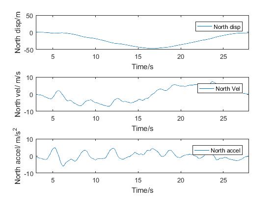
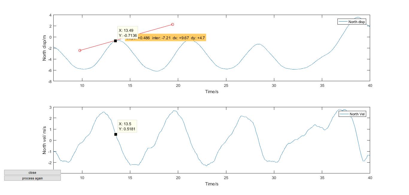
Pupils should execute this script by using the run button, top centre of the screen. They will be prompted to open a file. This file should be the one recorded in the lesson. After a short time, a graph similar to the one below, should appear:

In the graphs above, it can be noted, that the pupil started to run at 3 seconds and stopped at about 28 seconds.
This information is important.
In the command window, located at the bottom of the screen, pupils will be asked, “What time do you wish to start analysis from?” Pupils should enter a time in this window and hit the enter key. For the example above, they might add 3, and press enter. They will then be asked, “What time do you wish to end the analysis?”
28 seconds would be a reasonable time to end.
The programme will then perform its analysis. This may take a moment.
Eventually, matlab will produce a graph similar to the one below:
On the ‘figure’ screen, under the desktop ‘tab’ is the data-cursor icon.
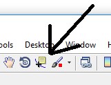
Pupils can click this to add a cursor point the graph’s curve. This will give them ‘x and y’ coordinates. In this case, Time and Displacement or Velocity. Multiple cursor points can be added by holding shift and re-clicking.
The shape of the graphs can be discussed with the pupils. They can then answer the questions on the reverse of ‘The Physics of sprinting’.
Intermediate
Go back to the file and to lines 399 to 411. These have been commented out but can be revived by clicking the green %x symbol at the top of the screen. Some lines will remain green – this is intentional.
Running the script again will give the pupils a quiver plot of the pupil’s velocity through time. See if the pupils can work out what they’re looking at and ask them to label the axes.
This is an excellent time to initiate a discussion on vectors.
Advanced
Gradients
Closing the most recent quiver plot students should open the file:
Getslopeintercept.m
This will open the most recent figure and ask the user to click on the graph. The pupils will be able to draw a tangent to the displacement/ time curve. The programme will then generate a value for the gradient. Using cursors as before, the pupils will be able to verify that the gradient of the distance time graph is the velocity at that instant. (This is useful as it highlights positive and negative gradients).
It is also possible, by de-commenting lines 386 – 390, to view the acceleration against/ time.
More pupils
It is likely that pupils will want to compare their V/t graphs… Welcome to the Vertigo project.
Pendulums
Investigating the periodic motion of a pendulum
Curriculum links
Key Stage 4 National Curriculum
-
interpreting quantitatively graphs of distance, time, and speed
-
acceleration caused by forces; Newton’s First Law
-
amplitude, frequency
Safety
appropriate risk assessment should be made in compliance with departmental requirements
Introduction
There are many ways to analyse the motion of a pendulum. This activity offers three different approaches of increasing complexity.
The beginner section looks at the acceleration Vertigo has experienced and offers a very simple determination of the Time period of oscillations.
The intermediate activity gives scope for pupils to investigate the relationship between displacement, velocity and acceleration.
The advanced analysis converts the data from a time domain into the frequency domain, introducing students to the Fourier transform and a means of presenting data they will likely not have encountered before.
Beginner
This analysis could fit into a wider study, perhaps investigating the relationship between pendulum length and Time period. It could also be used as a means of comparing data gathered by hand and by data loggers. The latter, ought to, in this case, yield a more accurate answer with smaller uncertainties.
Set-up
-
Tie Vertigo to a 1 metre length of light inextensible string (cotton thread would be best).
Although the GPS antenna will not be needed for this investigation, it does provide a convenient point to attach the string to, and so could still be connected to the vertigo board. -
Using two small pieces of wood, or a split cork, fix the other end of the string into a clamp. The clamp can then be connected to a retort stand as shown below.
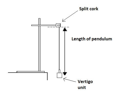
The length of the string is not too important but should be between 20cm and 1 metre. Measurng the length of the string should be from the bottom of the split cork to the centre of mass of the vertigo unit. This will involve some uncertainty. It may be useful to have pupils estimate this uncertainty and quote it in their results.
Data capture
-
Turn the vertigo device on
-
Wait for 30 seconds, keeping vertigo reasonably stationary
-
Press the log button to start logging
-
Displace vertigo to an angle of approximately 30 degrees and release
-
Allow Vertigo to perform 10 full swings
-
Stop the device and press the log button again.
If data acquisition fails, sample data is available for this activity here
Analysis
-
Remove the sd card from Vertigo and place it into a suitable sd card reader.
-
Open the programme matlab
-
The following files must be downloaded into a single folder Pendulum_scripts
-
In matlab, click the ‘open’ icon located in the top left of the screen, and navigate to the folder that has been downloaded. Open the file Pendulum_lesson.m
-
Click run
A graph will quickly appear that resembles the graph below:
In the command window, the operator will be asked
“Which orientation looks best? - North (1) or East (2)”
In the graph above the Blue line shows the clearest trend. This depends on which way the pendulum has been orientated. There will be a choice of either North or East as the pendulum has most amplitude in these directions.
Please enter, into the command window, a ‘1’ for North or a ‘2’ for East
The user will then be asked “when would you like to start the analysis?” Followed by:
“when would you like to end the analysis?”
Looking at the graph, it is clear that the less noisy oscillations occur beyond 4 seconds and end at around 16 seconds. Enter these values when prompted.
A new graph will then appear.
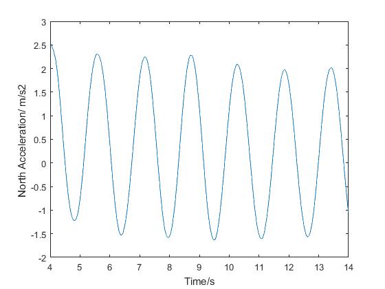
This graph can be used to determine the time-period of the pendulum.
For very accurate readings, the cursor icon
will allow pupils to find x/y values within 2 decimal places.
The time period for the pendulum above is
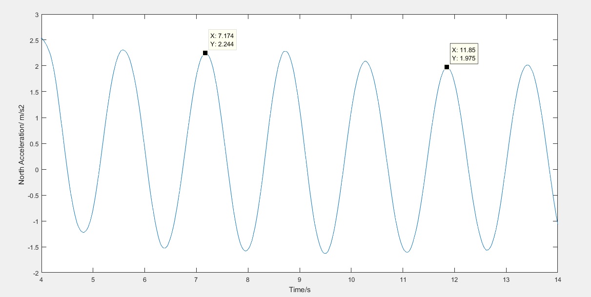
11.85s – 7.17s = 4.68 seconds for 3 full oscillations
Time Period = 4.68seconds/ 3 = 1.56 seconds
Giving a frequency of 0.64 Hz
This corresponds to a length of 60cm -which was exactly the length used.
Intermediate
In addition to investigating the Time period of the pendulum, its movement in the North and or East directions can be analysed.
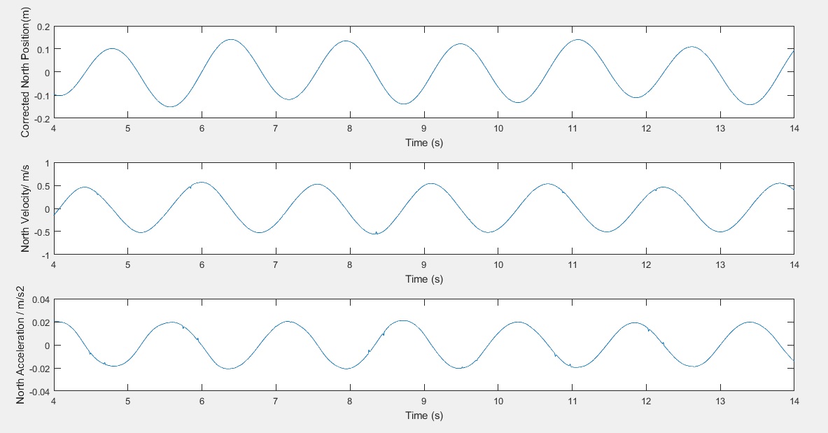
The Pendulum_lesson2 script can be used to produce a graph of displacement, Velocity and acceleration.
The script contains similar prompts as in the beginner exercise.
As before, in matlab, open the file Pendulum_lesson2
The final graph produced looks as follows
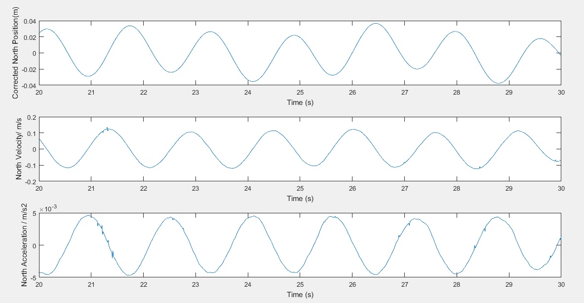
One point of interest, in this example, is to investigate the relationship between amplitude and time-period. Below is a graph from a second data set taken with the same pendulum but with a much-reduced amplitude. The isochronous nature of pendulums can be a conceptual hurdle, and some pupils find this difficult to overcome – it is very visible here.
Advanced
The final analysis is suitable for G&T students in years 11 or above. It involves understanding the moving of data from the time domain into the frequency domain.
The analysis should be used as an extension to the intermediate exercise and not as a stand-alone activity.
The script required is Pendulum_lesson3. Data should already have been loaded into Matlab with the previous scripts already complete.
(Note – this analysis gives a more accurate output if the data is recorded over a longer time frame. Leaving the pendulum to oscillate for over a minute would be ideal)
Notice, here, the peak amplitude occurs at a frequency of approximately 0.64 Hz which was the calculated frequency from earlier examples.
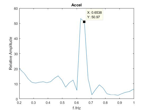
It is also interesting to note that whilst the pendulum will oscillate in the expected plane, it will also oscillate as a torsional pendulum. These frequencies often show themselves in the Fourier Transform. It may be an area worth investigating.
Circular Motion
The aim of this lesson is to support pupil understanding of circular motion and in particular centripetal force. Data should be taken outside, although there are options for lab-based experiments. Best outcomes are achieved when a constant radius, uniform speed circle is followed. This may be achieved by a pupil running, a pupil on a bicycle or other suitable vehicle.
The beginner section looks at the speed and velocity of the vertigo unit as it travels in a circle. The data presented in Distance/ time and a s a quiver plot.
The intermediate section looks at the same data but introduces the concept of acceleration.
The advanced section investigates the angle between the acceleration and the Velocity.
Beginner
Set-up
Suitably attached the Vertigo unit to the person or object that will be travelling in a circle. If possible, vertigo should be placed away from metal parts and be positioned such that its movement is as smooth as practically possible. (The metal may have some ferromagnetism that would affect vertigo’s the onboard magnetometer and any additional oscillatory motion would make pupil analysis more challenging)
-
Turn Vertigo on and wait for the second LED to stop flashing – Vertigo has a GPS signal.
-
Press the log button and ask the operator to perform circular motion for around 1 minute. Stop Vertigo’s logging.
Analysis
-
Remove the sd card from Vertigo and place it into a suitable sd card reader
-
Open the programme matlab
-
The following files must be downloaded into a single folder Circle_link_files
-
In matlab, click the ‘open’ icon located in the top left of the screen, and navigate to the folder that has been downloaded
-
Open the file Circular_lesson1
-
Click run
A graph similar to the one below will appear
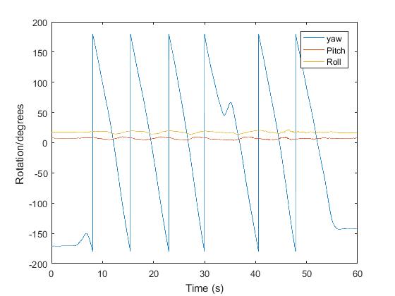
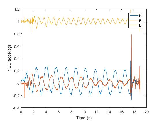
This shows how the angle Vertigo was orientated at changed through time. The most important in this instance is Yaw. It shows the angle Vertigo has moved through, around an imaginary vertical axis heading into the Earth. In this graph, it can be seen that Vertigo was travelling with a fairly constant angular velocity. (Notice that to make the graph easier to fit on a scale -180 degrees is converted into 180 degrees)
In the graph, Vertigo completes six full rotations – with a little wobble at 35 seconds. In order to keep the data as clean as possible for the pupils, it will is easier to look at one or two rotations only.
The operator will be asked –
“What time do you wish to start analysis from?” And then
“What time do you wish to end the analysis?”
For this data one rotation occurs between 8 and 16 seconds, and two rotations take place between 8 and 23 seconds.
Choosing between 8 and 16 seconds, the following graphs will appear:
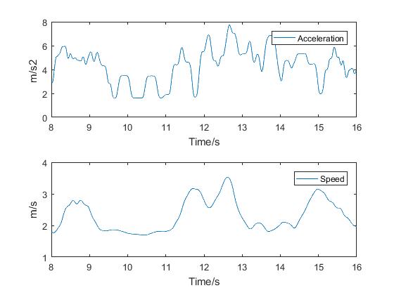
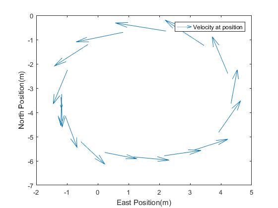
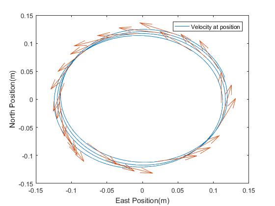
The latter shows the velocity of Vertigo at various positions as it travels in a circle. The critical point here is that the velocity is at a tangent to the direction.
The other graphs show how the speed varies. In this example, the data was taken on a slight slope and so the speed varies accordingly. It should be possible to achieve a fairly constant speed and this could be an activity for the pupils.
Intermediate
This activity looks to investigate the centripetal acceleration of an object travelling in a circle.
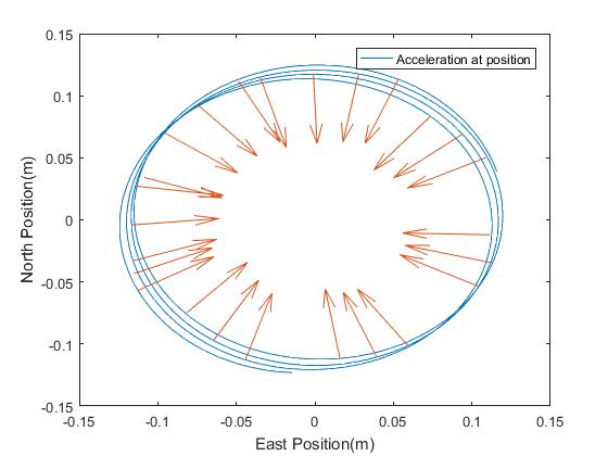
The first method is identical to the Beginner exercise with the addition of a quiver plot which shows acceleration at positions around the circle Vertigo travelled in.
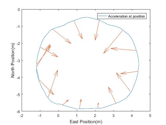
Ideally, this would point inwards. However, if the speed of the circular motion is not kept constant then there will be a component of acceleration in the direction of this increasing or decreasing speed. Depending on the class’s ability, this may be an interesting topic of discussion.
If a pure, textbook style centripetal acceleration is required, then Vertigo may be fitted to a fix speed turntable. An old record player works well.
If this is not available, data can be found here
Advanced
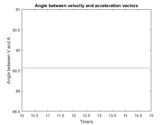
A more in-depth analysis could investigate the angle between the Velocity and Acceleration Vertigo experiences as it travels in a circle. This can be found be using the dot product of the two quiver vectors used in the previous lessons.
It would be expected that the angle between the velocity and acceleration would always be 90 degrees. As can be seen, this analysis reveals the angle to oscillate between 65 and 115 degrees.
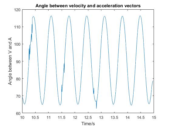
The average though is a little over 89.5 degrees – textbook. Why there is such variation could be an interesting area for investigation.
Trampoline Jumping

Beginner
Measuring the forces acting on a trampolinist.
For this experiment it will be assumed that the trampolinist is only moving in the vertical direction.
For consistency, and for ease of understanding, the trampolinist’s weight has been added on to the force charts.
Fix Vertigo onto the waist of the trampolinist – it is important that Vertigo is not landed on whilst jumping.
The GPS antenna is not needed.
- Turn vertigo on and keep it still for 30 seconds
- Press the log button
- Begin jumping
- Once finished, press the log button again to end the data capture.
- Wait until Vertigo’s LED lights stop flashing
The following Scripts need to be downloaded into the same folder
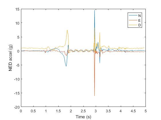
- Open matlab and run the script Trampoline_lesson_1
After a short time, a graph will appear.
NB
The data used here is not from a trampoline, but the scripts have been written for this purpose.
The operator will then be asked
- What time do you wish to start analysis from? In the command window normally found at the bottom of the matlab screen
Looking at the graph, input a suitable start time, in seconds, into the command window
And then:
- What time do you wish to end the analysis?
Chose an end time and enter this in seconds into the command window.
And finally
- What is the mass of the trampolinist?
This is simply required to calculate the force acting on the trampolinist using F=ma. Input the trampolinist’s mass in Kilograms.
Once this data has been entered, graphs such as the one below will be produced.
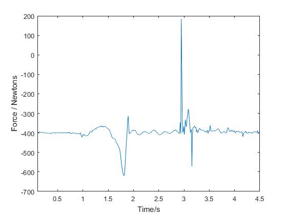
An interesting investigation could be to find the relationship between a pupil’s mass, and the maximum force experienced on the trampoline.
Intermediate
Force, displacement and velocity
It is also possible to investigate the height and velocity of the trampolinist. This is similar to previous investigations. The gradient of the distance/ time graph ought to be directly proportional to the velocity.
- Load the script Tramp_lesson2 and follow the instructions as before.
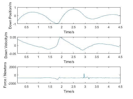
The final graph looks at the force that the trampoline exerts on the trampolinist as it is stretched. It is a difficult graph to analyse, if multiple jumps are viewed simultaneously.
- Adjusting the ‘force window’ required can be achieved by modifying line 137 of the matlab script.
ylim([150 300]);
Change the limits, in the square brackets, to ones more applicable to your investigation.
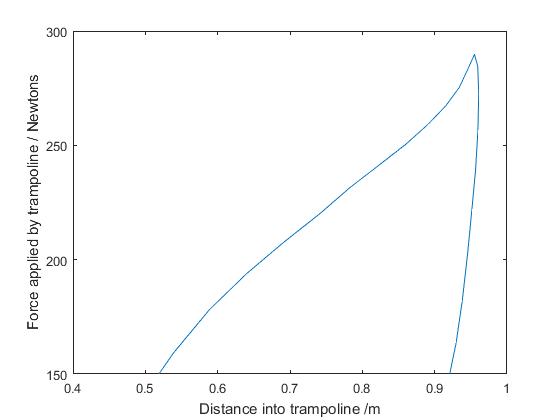
It is possible, though reasonably involved, to investigate the energy stored in the trampoline.
Advanced
Measuring rotation
When measuring rotational speeds, the frame of reference is all important.
Similar to concepts in relativity, the need to stipulate the frame used is important.
Linear speed is most often measured with respect to longitude and latitude coordinates on the Earth’s surface. But this might not be as valuable to a plane or a boat, where speed, in relation to the air or water, is more important.
The same is true when measuring the rotational speeds for a trampolinist.
 |
 |
|---|---|
| A ‘NED’ world frame | How a Board frame may be assigned |
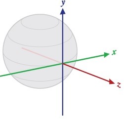
The diagram on the left shows a ‘world frame’. That is, one that has axes fixed to the Earth. Convention has X,Y and -Z following the directions of North, East and Down (NED).
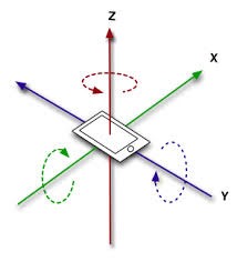
The diagram on the right shows rotational axes that rotate with the object. In this particular case, Vertigo will be fixed onto a rotating trampolinist.
For this investigation, the rotating frame will be most useful. And therefore, for the first, and possible only time, the orientation with which Vertigo is attached to the trampolinist will be important. Especially, if results between trampolinists are to be compared.
Load the script trampoline_lesson3
Acquire data as before and follow instructions in the command window. Several graphs will appear, all with labelled axes to ease understanding.
Visualising rotations in 3-dimentions can be challenging, and it will take some time to be confident in explaining what the graphs represent. The following graphs help to understand the problems involved.
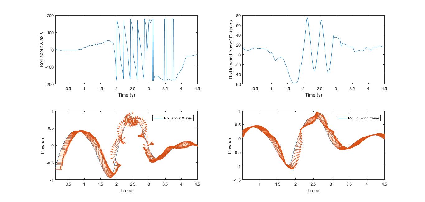
Roll Rotations
Pitch Rotations
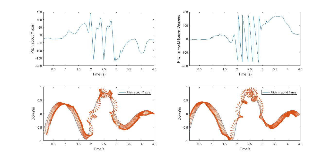
Rotations can be seen in both the world frame and the trampolinist’s frame of reference. What appears to have happened, in this example, is that the board’s X-axis was rotating about an imaginary axis running across the Earth, East to West.
The other oscillations are presumably processional.
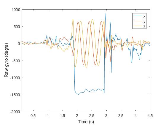
The oscillation direction can also be seen from the gyroscope rate. In the graph below, it is clear the most rotations is occurring around the x-axis.
It should be clear that, if rotations between athletes are to be compared, Vertigo will need to be affixed in a consistent manner. Or, the trampoline jumper would need to face the same way each time he/she jumped.
NB
The data used here was obtained by throwing a Vertigo upward and then catching it. The first throw was launched with little spin, the second with a higher revolution rate. These rates would be much higher than a trampolinist might achieve.
Comparing the results, measured with Vertigo, against a video recording of a trampolinist, would be a very interesting exercise.
Since angular momentum is always conserved, the rate of rotation can be increased as the trampolinist varies their moment of inertia. (This is not the case with the ‘board thrown in the air’ data presented here).